Vision-based control of the plane Poiseuille flow

Contact :

Roméo Tatsambon Fomena, Christophe Collewet

Description

We proposed in [Tatsambon and Collewet, 2011a; Tatsambon and Collewet, 2011d] a new approach to control a flow. Controlling a flow consists either to change its state to another state or to maintain its current state whatever external disturbances by acting on this flow. Here the control of the laminar plane Poiseuille flow by blowing and suction is considered. To estimate the state of this flow, existing control methods rely on a set of limited wall shear stress measurements. However, those methods suffer from limited observations, from noisy measurements and from the initialization process involved in the observer required to estimate the flow state. To deal with these issues, we proposed a vision-based control approach. More precisely, by visualizing a fluid flow, dense flow velocity maps can be computed via optical flow techniques (see for example [Champagnat et al., 2009]) and subsequently used to build an observer-free closed-loop control law. This approach is formally proven to be of great improvements for the control of this flow in comparison with existing control approaches.

Plane Poiseuille flow

Poiseuille flow is a flow in an infinite length channel due to a pressure gradient. This flow has become a standard problem to develop flow control theories. One of the main reason is that the analytical solution to the Navier-Stokes equations of the steady state Poiseuille flow is well-kown in fluid mechanics. The steady state velocities profile is illustrated on Fig. 1. The x-axis is associated to the streamwise direction, the y-axis to the normal direction and the z-axis to the spanwise direction of the flow.

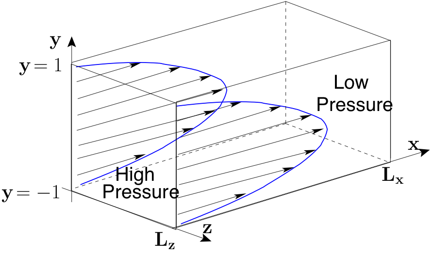Fig. 1. Steady state velocities profile of a 3D plane Poiseuille flow (L_x and L_z are the period lengths assuming a periodic flow).

Most of the works focus on temporal instabilities caused by a perturbation velocity. In order to keep permanent such instabilities in the infinite channel when the flow is not controlled, a periodic boundary finite length channel is assumed (see Fig. 1). That is why the perturbation velocity can be expanded in a Fourier series. Thereafter, the fundamental wavenumber pair (α_n, β_n) is introduced.

Control principle

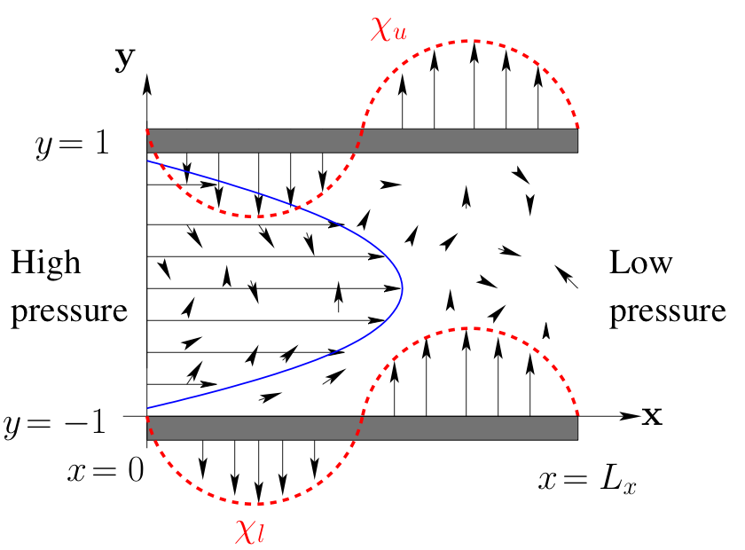
This flow can be controlled via boundaries. Boundary control consists in modifying boundaries conditions either only on the lower boundary y = -1, or on both the upper y = 1 and lower y = -1 boundaries. From a physical point of view, boundary control can be interpreted as a geometric alteration of the boundary as pictured on Fig. 2. The boundary control on the upper and the lower channels can be theoretically modeled by functions χ_u and χ_l that ensure mass conservation in the controlled system as pictured on Fig. 2. Note that in the absence of control, i.e. when χ_u = χ_l = 0, the red dashed curves (see Fig. 2) are aligned with the lower and upper boundary lines as expected.

Fig. 2. Boundaries control of the plane Poiseuille flow.

Reduced linearized model

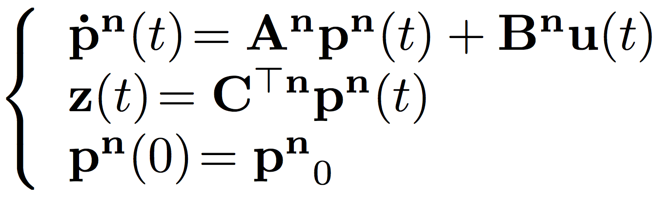
For a pratical implementation of flow control methods, the infinite dimension of a flow prompts the need for a reduced flow model. The modeling consists first of all in linearizing the Navier-Stokes equations (NSE) around the steady state solution. Then the continuous linearized model of the NSE is reduced by approximation of the perturbation velocity at a spefically selected wavenumber pair (α_n, β_n) of the Fourier series and by decomposition of the specifically selected Fourier series coefficients through the evaluation of combinations of Chebychev polynomials at Gauss-Lobatto collocation points y_k. Finally, the null boundary conditions of the closed-loop control system is obtained by setting the upper and lower boundaries to the values of the control inputs χ_u and χ_l respectively. All computation done, the reduced linearized model is given by the following canonical expression:

(1)

where pⁿ(t) is the state vector, Aⁿ is the state matrix, u(t) is the system control inputs on the upper and lower channel boundaries, Bⁿ is the input matrix, Cⁿ is the output matrix and z(t) is the vector of shear stress measurements on the upper and lower boundaries.

Control law

The most classical way to control the plane Poiseuille flow uses a Linear Quadratic Gaussian (LQG) controller. This approach is based on an estimated value of the state vector pⁿ(t) which is obtained from the shear stress measurements using an observer built from a Linear Quadratic Estimation scheme. However, as will be proven in the next section, an observer is sensitive to its initialization and converges asymptotically to the true flow state value. Moreover, because of limited observations, noisy measurements produce noisy flow state estimated values. Both of these issues are not suitable in the framework of flow control since a poor and noisy estimated state used in a control law could trigger transition to turbulence in the controlled flow and therefore might cause the divergence of the control law.

The control signal for the output feedback LQG controller is then:

Expression of the output feedback LQG controller

(2)

where vector k is the LQG optimal gain; the second vector is an estimated value of the state vector pⁿ(t). This control law (2) will be refer to as shear stress based LQG (SSB-LQG) control.

Another way to proceed is to estimate the state vector from visual features obtained from a vision system sensing the flow. More precisely, the optical flow is used. A key point in vision-based control is that this control technique belongs to the class of sensor-based control of dynamic systems: the control law is computed in the sensor frame. Consequently, this approach corresponds clearly to an observer-free feedback control. Another great advantage of such a sensor is that it is non-intrusive. This sensor is also an extremely rich and dense source of information on the flow. We will refer to this vision-based control law as the vision-based LQG (VB-LQG) control law since the state is obtained from visual measurements instead of shear stress measurements as used in (2).

Results

Vision-based control of an unstable flow in the ideal case

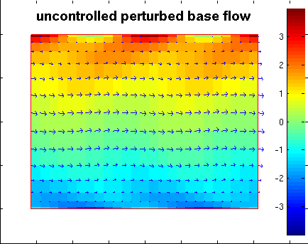
For the Reynolds number Re = 10 000 and the wavenumber pair (α_n = 1, β_n = 0),the flow presents. In this case the flow is initially in the steady state but in an unstable equilibrium, i.e. a small disturbance velocity value destabilizes the uncontrolled fluid flow.

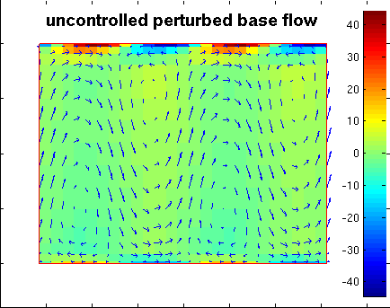
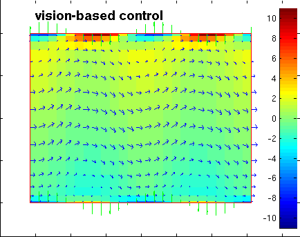
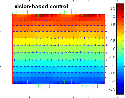
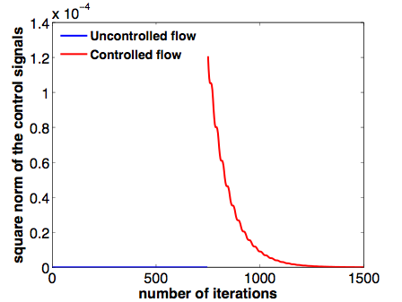
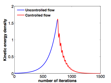
We first present results concerning the VB-LQG control approach in the ideal case where there is no measurements noise. Fig. 3 shows the different steps in the control of the perturbed flow. Fig. 3(a) pictures the desired image of the flow corresponding to the steady state velocities profile; Fig. 3(b) shows the image of the flow just before the application of the vision-based control law where we can see that the flow has become turbulent. Figs. 3(c) and 3(d) show different steps of the controlled flow at arbitrary selected iteration numbers k = 1047 and k = 1500 respectively: the control at each selected instant is represented by green vertical arrows on the upper and the lower channel boundaries. The control law converges since it tends towards 0 as shown on Fig. 3(e). Moreover, Fig. 3(f) depicts the kinetic energy density of the flow perturbation where we can see an increase due to the pertubation growth in the case where the flow is not controlled; and then a decrease also towards 0 once the control law is applied. At this step, we can see that the final velocities profile given in Fig. 3(d) is very similar to the desired velocities profile in Fig. 3(a).

Fig. 3. Vision-based control (the color in the figures represents the vorticity map). (a) desired image of the flow; (b) initial image of the flow, the perturbation has grown k= 750; (c) controlled flow at k = 1047; (d) controlled flow at k = 1500; (e) Control law versus frame iteration and (f) kinetic energy density versus frame iteration; (g) video.

(a)	(b)

(c)	(d)

(e)	(f)

(g)

Comparison of the estimation methods

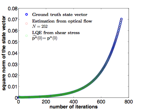
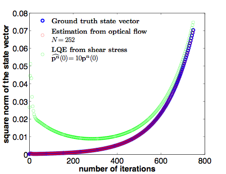
Here we show that the vision-based state estimation provides better results than the Linear Quadratic Estimation (LQE) scheme state estimation usually used. We consider a perturbed flow that is not controlled. Results are given in Fig. 4 in terms of the square norm of the state vector. Fig. 4(a) presents the ideal case where there is no measurements noise and no initialization error. From this figure we can see that both estimations perfectly correspond to the ground truth value of the state vector. Fig. 4(b) highlights the poor initialization issue and the asymptotic convergence issue in the LQE; these issues are not of concerned in the vision-based approach which provides the ground truth value of the state vector as shown in [Tatsambon and Collewet, 2011a; Tatsambon and Collewet, 2011d].

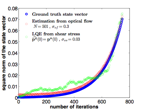
The robustness to noise of the vision-based state estimation is presented on Fig. 4(c) where the standard deviation (STD) σ_of on the optical flow noise has been purposely set to a value 10 times higher than the STD σ_ss on the shear stress noise. This figure presents an average over a large number of realizations of the stochastic noises in the case where N = 501 pixels are used. Note that N = 501 is far less than the number of pixels available in real situations where the images size can be at least 1280 x 960 (N = 1280) (the more N is high, the less the estimated value of the state is sensitive to noise [Tatsambon and Collewet, 2011a; Tatsambon and Collewet, 2011d]). Due to a large number of flow particles velocities provided by visual sensing, the new approach is very robust to noisy measurements.

All those result confirm that the vision-based estimation performs better than the LQE from shear stress measurements in any case.

Fig. 4. Comparison of state vector estimations using shear stress and optical flow: (a) ideal case; (b) LQE poor initialization; (c) measurements noise for a given number of pixels N.

(a)	(b)	(c)

Behavior of the closed-loop systems

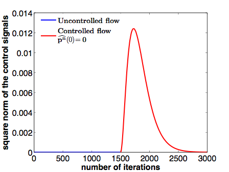
The behavior of the closed-loop system is shown to be better with the VB-LQG approach than with the SSB-LQG approach. Results are presented in Fig. 5. Fig. 5(a) depicts the behavior of the control signal in the ideal case (no measurements noise, no initialization error). Fig. 5(b) depicts the behavior of the control signal when the initial value of the estimation of the state is set as 0 by default since this value is unknown. In this case we can see that the value of the control signal is 100 times higher than the ideal control signal case which includes the VB-LQG approach (compare the highest control signal values in Fig. 5(a) and Fig. 5(b)). This higher control signal value could lead to an unsuitable state trajectory which can cause the real non-linear system to diverge. In addition, as expected, the control signal (see Fig. 5(b)) takes more time to converge to 0 (3000 iterations compared to the VB-LQG approach). This leads to an energy consumption far much higher for the SSB-LQG control than for the VB-LQG control.

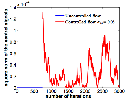
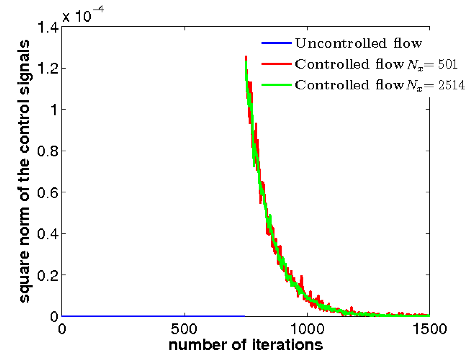
The second row of Fig. 5 presents the control signals in presence of measurements noise. Fig. 5(c) pictures the case of the SSB-LQG control where we can see that the control signal does not converge to zero: although the noise STD has been set to a small value σ_ss, the control signal is very noisy, which is not suitable for actuators. Finally, Fig. 5(d) illustrates the robustness of the VB-LQG control where the STD in the optical flow noise is 10 times higher than the STD in the shear stress noise: we can see from this last figure that the larger the sample of flow particles velocities used the lesser the noise in the control signal.

Fig. 5. Comparison between the SSB-LQG and the VB-LQG control signals: (a) ideal case (no measurements noise, no initialization error); (b) initialization error in the SSB-LQG approach; (c) measurements noise the SSB-LQG approach; (d) measurements noise in the VB-LQG approach.

(a)	(b)

(c)	(d)

Reduction of the transient energy growth

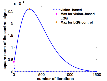
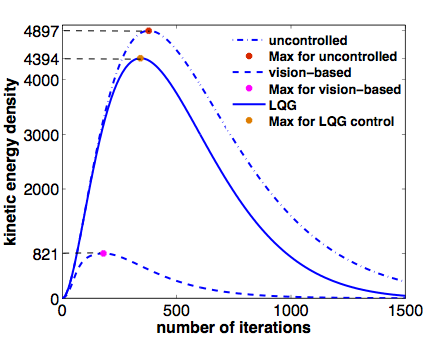
In the case where the Reynolds number is set to Re = 5 000 and the wavenumber pair is set to (α_n = 0, β_n = 2.044) the reduced linearized system is stable. However, in this case, it is possible to find the worst initial condition which causes the reduced linearized system to present the maximum transient energy growth. In this case, if the flow is not controlled the high transient energy could instigate transition to turbulence in the real flow. Therefore, the goal of the control law (2) is now to reduce as far as possible the value of this maximum.

Let pⁿ_worst(0) be the initial condition corresponding the maximum transient energy growth showed with the red dot on the blue dash-dotted plot on Fig. 6(b) in the case where the flow is not controlled. We consider the VB-LQG and the SSB-LQG approaches in the ideal case where there is no measurements noise. In addition, we assume reasonable to set zero observer initial conditions for the SSB-LQG controller. Fig. 6(a) shows the behavior of the control signals, as can be seen the maximun control value for the SSB-LQG is 5 times the maximum control value of the VB-LQG approach. On Fig. 6(b) we can see that the kinetic energy is much more reduced by the VB-LQG controller than by the SSB-LQG control. This is mainly due to the asymptotic convergence of the observer used in the SSB-LQG approach. To sum up, the VB-LQG controller offers a better reduction of the kinetic energy density with much lesser control efforts than the SSB-LQG controller.

Fig. 6. VB-LQG and SSB-LQG controls for the worst initial conditions: (a) control signals; (b) kinetic energy density.

(a)	(b)

Conclusion

In this demo we have shown the efficiency of a vision-based approach for fluid flows control. This approach uses image measurements to estimate the flow state. Results have been presented to show the improvements on state estimation and flows control provided by the vision-based approach over the commonly proposed shear stress based LQG control. Indeed the shear stress based LQG regulator limitations concern the limited number of shear stress measurements, the measurements noise and the initialization of the observer involved in the flow state estimation. The initialization issue is not of concerned in the vision-based approach. In addition the vision-based approach has been shown to be robust to measurements noise since a large number of flow velocities is available in real practical situations.

References

R. Tatsambon Fomena, C. Collewet. Fluid Flows Control using Visual Servoing. In: 18th IFAC World Congress, Pages 3142-3147, Milan, Italy, September 2011.
R. Tatsambon Fomena, C. Collewet. Vision-based Control of 2D Plane Poiseuille Flow. In: 7th Int. Symp. on Turbulence and Shear Flow Phenomena, TSFP-7, Ottawa, Canada, July 2011.